K Nearest Neighbors

Description:

You’ve been given a classified data set from a company! They’ve hidden the feature column names but have given you the data and the target classes.

Use KNN to create a model that directly predicts a class for a new data point based off of the features.

Import Libraries

import pandas as pd
import seaborn as sns
import matplotlib.pyplot as plt
import numpy as np
%matplotlib inline
from sklearn.preprocessing import StandardScaler
from sklearn.model_selection import train_test_split
from sklearn.neighbors import KNeighborsClassifier
from sklearn.metrics import classification_report,confusion_matrix

Get the Data

df = pd.read_csv("./../../data/Classified Data", index_col=0)

df.head()

	WTT	PTI	EQW	SBI	LQE	QWG	FDJ	PJF	HQE	NXJ	TARGET CLASS
0	0.913917	1.162073	0.567946	0.755464	0.780862	0.352608	0.759697	0.643798	0.879422	1.231409	1
1	0.635632	1.003722	0.535342	0.825645	0.924109	0.648450	0.675334	1.013546	0.621552	1.492702	0
2	0.721360	1.201493	0.921990	0.855595	1.526629	0.720781	1.626351	1.154483	0.957877	1.285597	0
3	1.234204	1.386726	0.653046	0.825624	1.142504	0.875128	1.409708	1.380003	1.522692	1.153093	1
4	1.279491	0.949750	0.627280	0.668976	1.232537	0.703727	1.115596	0.646691	1.463812	1.419167	1

df.info()

<class 'pandas.core.frame.DataFrame'>
Index: 1000 entries, 0 to 999
Data columns (total 11 columns):
 #   Column        Non-Null Count  Dtype
---  ------        --------------  -----
 0   WTT           1000 non-null   float64
 1   PTI           1000 non-null   float64
 2   EQW           1000 non-null   float64
 3   SBI           1000 non-null   float64
 4   LQE           1000 non-null   float64
 5   QWG           1000 non-null   float64
 6   FDJ           1000 non-null   float64
 7   PJF           1000 non-null   float64
 8   HQE           1000 non-null   float64
 9   NXJ           1000 non-null   float64
 10  TARGET CLASS  1000 non-null   int64
dtypes: float64(10), int64(1)
memory usage: 93.8 KB

Standardize the Variables

Because the KNN classifier predicts the class of a given test observation by identifying the observations that are nearest to it, the scale of the variables matters. Any variables that are on a large scale will have a much larger effect on the distance between the observations, and hence on the KNN classifier, than variables that are on a small scale.

scaler = StandardScaler()
scaler.fit(df.drop('TARGET CLASS',axis=1))

StandardScaler()

In a Jupyter environment, please rerun this cell to show the HTML representation or trust the notebook.
On GitHub, the HTML representation is unable to render, please try loading this page with nbviewer.org.

scaled_features = scaler.transform(df.drop('TARGET CLASS',axis=1))

df_feat = pd.DataFrame(scaled_features,columns=df.columns[:-1])
df_feat.head()

	WTT	PTI	EQW	SBI	LQE	QWG	FDJ	PJF	HQE	NXJ
0	-0.123542	0.185907	-0.913431	0.319629	-1.033637	-2.308375	-0.798951	-1.482368	-0.949719	-0.643314
1	-1.084836	-0.430348	-1.025313	0.625388	-0.444847	-1.152706	-1.129797	-0.202240	-1.828051	0.636759
2	-0.788702	0.339318	0.301511	0.755873	2.031693	-0.870156	2.599818	0.285707	-0.682494	-0.377850
3	0.982841	1.060193	-0.621399	0.625299	0.452820	-0.267220	1.750208	1.066491	1.241325	-1.026987
4	1.139275	-0.640392	-0.709819	-0.057175	0.822886	-0.936773	0.596782	-1.472352	1.040772	0.276510

Train Test Split

X_train, X_test, y_train, y_test = train_test_split(scaled_features,df['TARGET CLASS'],
                                                    test_size=0.30)

Using KNN

Remember that we are trying to come up with a model to predict whether someone will TARGET CLASS or not. We’ll start with k=1.

knn = KNeighborsClassifier(n_neighbors=1)

knn.fit(X_train,y_train)

KNeighborsClassifier(n_neighbors=1)

In a Jupyter environment, please rerun this cell to show the HTML representation or trust the notebook.
On GitHub, the HTML representation is unable to render, please try loading this page with nbviewer.org.

pred = knn.predict(X_test)

Predictions and Evaluations

print(confusion_matrix(y_test,pred))

[[140  15]
 [ 14 131]]

print(classification_report(y_test,pred))

              precision    recall  f1-score   support

           0       0.91      0.90      0.91       155
           1       0.90      0.90      0.90       145

    accuracy                           0.90       300
   macro avg       0.90      0.90      0.90       300
weighted avg       0.90      0.90      0.90       300

Choosing a K Value

Use the elbow method to pick a good K Value:

error_rate = []

# Will take some time
for i in range(1,40):

    knn = KNeighborsClassifier(n_neighbors=i)
    knn.fit(X_train,y_train)
    pred_i = knn.predict(X_test)
    error_rate.append(np.mean(pred_i != y_test))

plt.figure(figsize=(10,6))
plt.plot(range(1,40),error_rate,color='blue', linestyle='dashed', marker='o',
         markerfacecolor='red', markersize=10)
plt.title('Error Rate vs. K Value')
plt.xlabel('K')
plt.ylabel('Error Rate')

Text(0, 0.5, 'Error Rate')

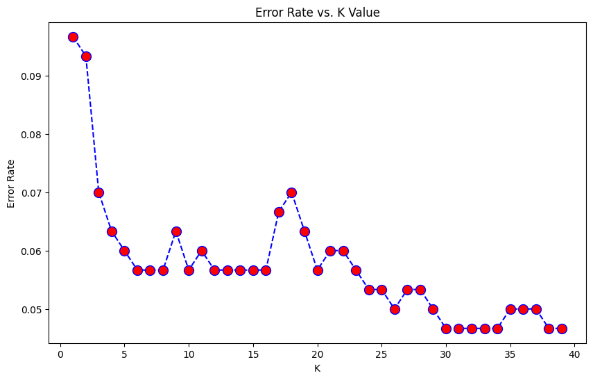
Here we can see that that after arouns K>23 the error rate just tends to hover around 0.06-0.05 Let’s retrain the model with that and check the classification report!

# FIRST A QUICK COMPARISON TO OUR ORIGINAL K=1
knn = KNeighborsClassifier(n_neighbors=1)

knn.fit(X_train,y_train)
pred = knn.predict(X_test)

print('WITH K=1')
print('\n')
print(confusion_matrix(y_test,pred))
print('\n')
print(classification_report(y_test,pred))

WITH K=1


[[140  15]
 [ 14 131]]


              precision    recall  f1-score   support

           0       0.91      0.90      0.91       155
           1       0.90      0.90      0.90       145

    accuracy                           0.90       300
   macro avg       0.90      0.90      0.90       300
weighted avg       0.90      0.90      0.90       300

# NOW WITH K=23
knn = KNeighborsClassifier(n_neighbors=23)

knn.fit(X_train,y_train)
pred = knn.predict(X_test)

print('WITH K=23')
print('\n')
print(confusion_matrix(y_test,pred))
print('\n')
print(classification_report(y_test,pred))

WITH K=23


[[141  14]
 [  3 142]]


              precision    recall  f1-score   support

           0       0.98      0.91      0.94       155
           1       0.91      0.98      0.94       145

    accuracy                           0.94       300
   macro avg       0.94      0.94      0.94       300
weighted avg       0.95      0.94      0.94       300