Linear regression
Description:
Make an ML algorithm to predict the house prices based on house features such as:
Avg. Area Income: Avg. Income of residents of the city house is located in.
Avg. Area House Age: Avg Age of Houses in same city
Avg. Area Number of Rooms: Avg Number of Rooms for Houses in same city
Avg. Area Number of Bedrooms: Avg Number of Bedrooms for Houses in same city
Area Population: Population of city house is located in
Price: Price that the house sold at
Address: Address for the house
Import
[32]:
import pandas as pd
import numpy as np
import matplotlib.pyplot as plt
import seaborn as sns
from sklearn.model_selection import train_test_split
from sklearn.linear_model import LinearRegression
from sklearn import metrics
Load the data
[46]:
USAhousing = pd.read_csv(r'./../../data/USA_Housing.csv')
Data exploration
[34]:
USAhousing.info()
<class 'pandas.core.frame.DataFrame'>
RangeIndex: 5000 entries, 0 to 4999
Data columns (total 7 columns):
 #   Column                        Non-Null Count  Dtype
---  ------                        --------------  -----
 0   Avg. Area Income              5000 non-null   float64
 1   Avg. Area House Age           5000 non-null   float64
 2   Avg. Area Number of Rooms     5000 non-null   float64
 3   Avg. Area Number of Bedrooms  5000 non-null   float64
 4   Area Population               5000 non-null   float64
 5   Price                         5000 non-null   float64
 6   Address                       5000 non-null   object
dtypes: float64(6), object(1)
memory usage: 273.6+ KB
[35]:
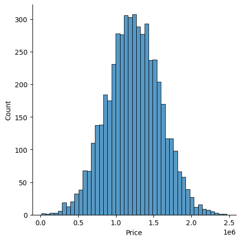
sns.displot(USAhousing['Price'])
[35]:
<seaborn.axisgrid.FacetGrid at 0x229d2af7ee0>
[36]:
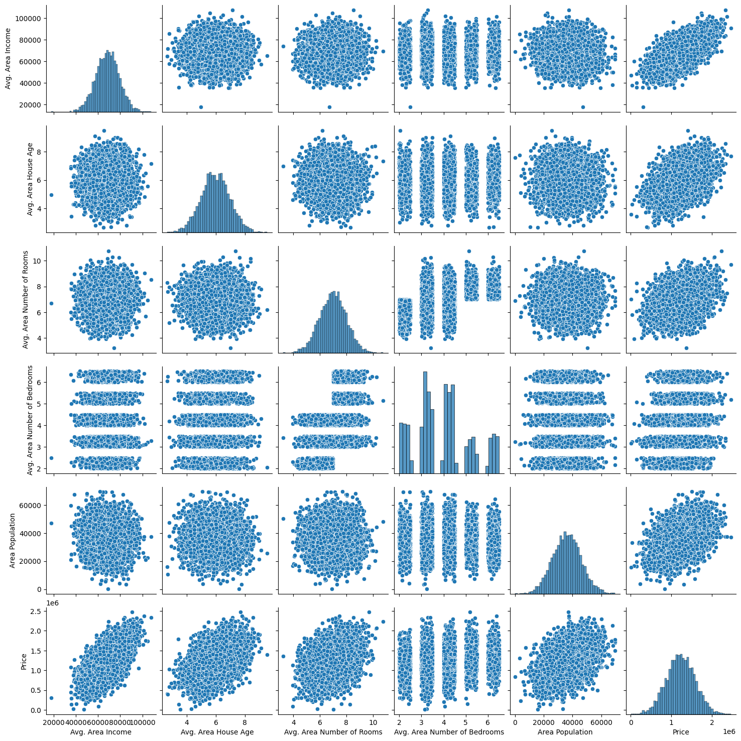
sns.pairplot(USAhousing)
[36]:
<seaborn.axisgrid.PairGrid at 0x229d1ffff70>
[37]:
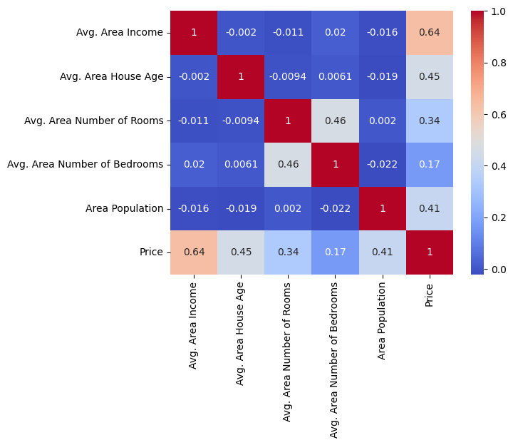
df_corr = USAhousing.select_dtypes(include=np.number).corr()
sns.heatmap(df_corr, cmap="coolwarm", annot=True)
[37]:
<Axes: >
Festures selection and data split
[38]:
#Houses features
X = USAhousing[['Avg. Area Income', 'Avg. Area House Age', 'Avg. Area Number of Rooms',
       'Avg. Area Number of Bedrooms', 'Area Population']]

#Prices that the modell needs to determine
Y = USAhousing['Price']
[39]:
X_train, X_test, y_train, y_test = train_test_split(X, Y, test_size=0.4, random_state=101)
Modell training
[40]:
#train the modell
lm = LinearRegression()
lm.fit(X_train, y_train)
[40]:
LinearRegression()In a Jupyter environment, please rerun this cell to show the HTML representation or trust the notebook.
On GitHub, the HTML representation is unable to render, please try loading this page with nbviewer.org.
LinearRegression()
Model evaluation
[41]:
#get the coefficient
print(lm.intercept_) # ??
lm.coef_
cdf = pd.DataFrame(lm.coef_, X.columns, columns=['Coeff'])
cdf
-2640159.796852963
[41]:
| Coeff | |
|---|---|
| Avg. Area Income | 21.528276 |
| Avg. Area House Age | 164883.282027 |
| Avg. Area Number of Rooms | 122368.678027 |
| Avg. Area Number of Bedrooms | 2233.801864 |
| Area Population | 15.150420 |
Interpreting the coefficients:
Holding all other features fixed, a 1 unit increase in Avg. Area Income is associated with an increase of $21.52 .
Holding all other features fixed, a 1 unit increase in Avg. Area House Age is associated with an increase of $164883.28 .
etc…
Prediction
[42]:
#prediction
predictions = lm.predict(X_test)
Results visualisation
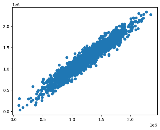
[43]:
plt.scatter(predictions, y_test)
[43]:
<matplotlib.collections.PathCollection at 0x229d6f9bdc0>
[44]:
sns.displot(y_test-predictions) #it should be a normal distribution
[44]:
<seaborn.axisgrid.FacetGrid at 0x229d01b4970>

Results evaluation
Here are three common evaluation metrics for regression problems:
Mean Absolute Error (MAE) is the mean of the absolute value of the errors:
Mean Squared Error (MSE) is the mean of the squared errors:
Root Mean Squared Error (RMSE) is the square root of the mean of the squared errors:
Comparing these metrics:
MAE is the easiest to understand, because it’s the average error.
MSE is more popular than MAE, because MSE “punishes” larger errors, which tends to be useful in the real world.
RMSE is even more popular than MSE, because RMSE is interpretable in the “y” units.
All of these are loss functions, because we want to minimize them.
[45]:
print('MAE:', metrics.mean_absolute_error(y_test, predictions))
print('MSE:', metrics.mean_squared_error(y_test, predictions))
print('RMSE:', np.sqrt(metrics.mean_squared_error(y_test, predictions)))
MAE: 82288.22251914945
MSE: 10460958907.208805
RMSE: 102278.82922290813