Logistic Regression
Description:
Build a ML classification algorithm to predict if the titatnic passenger will survive or not based on the passenger features:
Import Libraries
[75]:
import pandas as pd
import numpy as np
import matplotlib.pyplot as plt
import seaborn as sns
%matplotlib inline
from sklearn.model_selection import train_test_split
from sklearn.linear_model import LogisticRegression
from sklearn.metrics import classification_report
Load the data
[76]:
train = pd.read_csv(r"./../../data/titanic_train.csv")
Data Exploration
[77]:
train.info()
<class 'pandas.core.frame.DataFrame'>
RangeIndex: 891 entries, 0 to 890
Data columns (total 12 columns):
 #   Column       Non-Null Count  Dtype
---  ------       --------------  -----
 0   PassengerId  891 non-null    int64
 1   Survived     891 non-null    int64
 2   Pclass       891 non-null    int64
 3   Name         891 non-null    object
 4   Sex          891 non-null    object
 5   Age          714 non-null    float64
 6   SibSp        891 non-null    int64
 7   Parch        891 non-null    int64
 8   Ticket       891 non-null    object
 9   Fare         891 non-null    float64
 10  Cabin        204 non-null    object
 11  Embarked     889 non-null    object
dtypes: float64(2), int64(5), object(5)
memory usage: 83.7+ KB
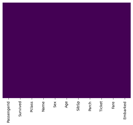
[78]:
sns.heatmap(train.isnull(),yticklabels=False,cbar=False,cmap='viridis')
[78]:
<Axes: >
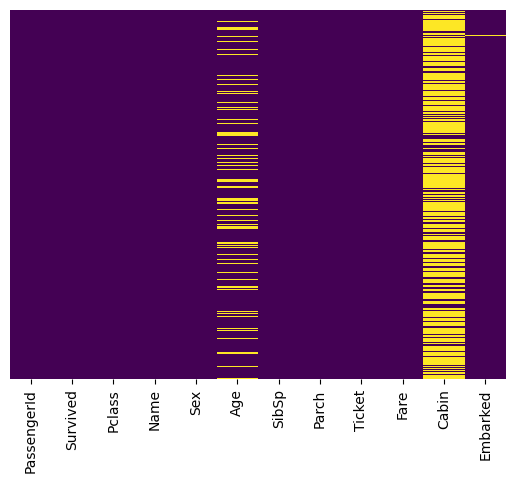
Handling NaN values
Remove ‘Cabin’ columns beceause of it has too much NaN to be filled/interpoled
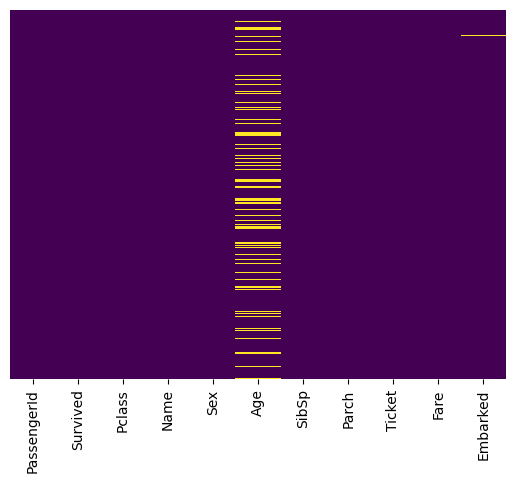
[79]:
train.drop('Cabin', axis=1, inplace=True)
sns.heatmap(train.isnull(),yticklabels=False,cbar=False,cmap='viridis')
[79]:
<Axes: >
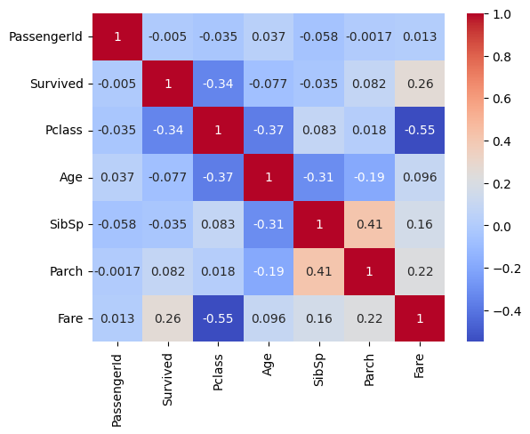
[80]:
df_corr = train.select_dtypes(include=np.number).corr()
sns.heatmap(df_corr, cmap="coolwarm", annot=True)
[80]:
<Axes: >
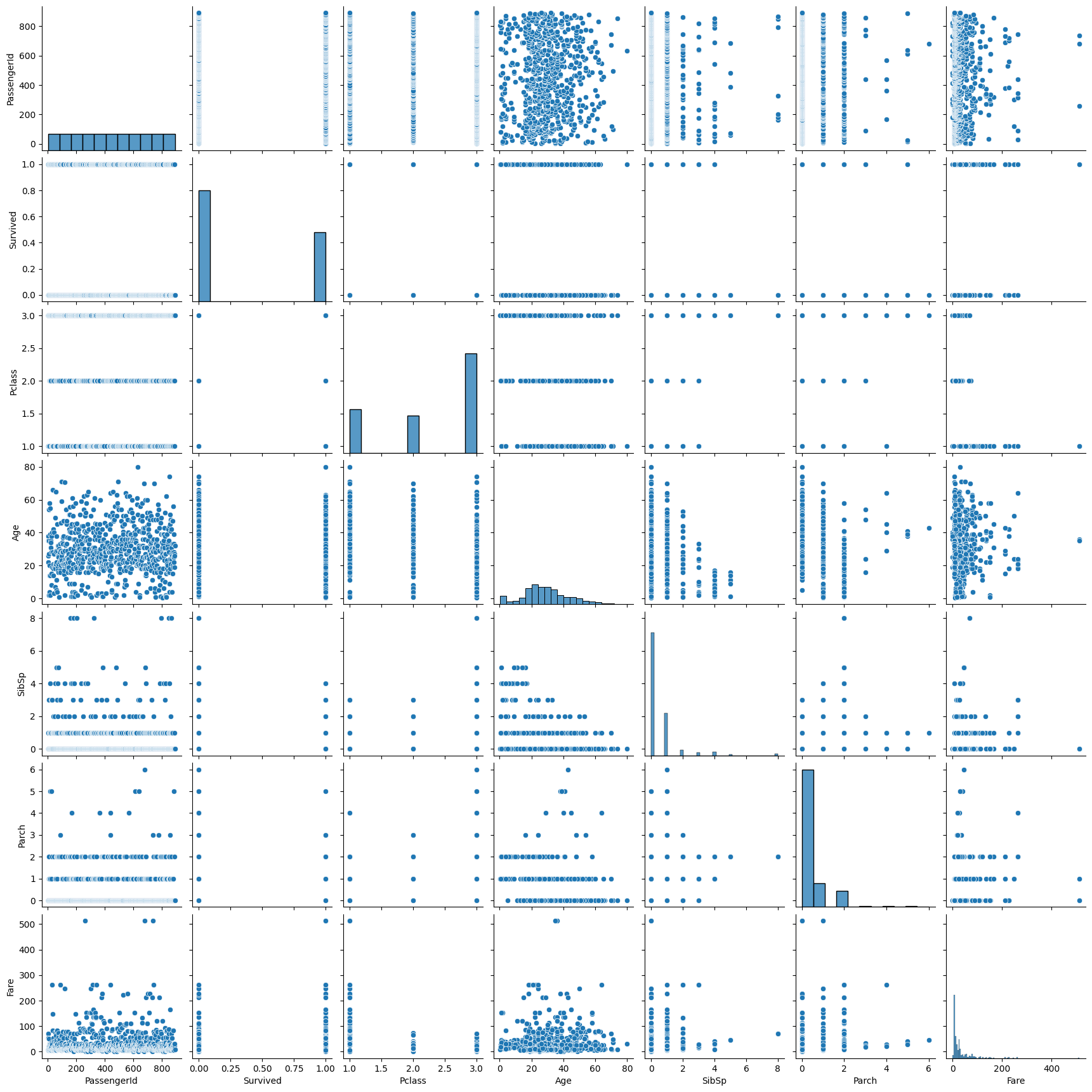
[81]:
sns.pairplot(train)
[81]:
<seaborn.axisgrid.PairGrid at 0x23ba66701f0>
[82]:
sns.boxplot(data=train, y='Age', x="Pclass")
[82]:
<Axes: xlabel='Pclass', ylabel='Age'>
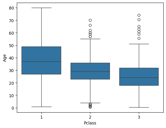
[83]:
pd_classe_age = train.groupby("Pclass")['Age'].mean().astype(int)
[84]:
def fill_age(row):
    if np.isnan(row['Age']):
        row['Age'] = pd_classe_age.loc[row['Pclass']]
    return row

train = train.apply(fill_age, axis=1)
sns.heatmap(train.isnull(),yticklabels=False,cbar=False,cmap='viridis')
[84]:
<Axes: >

[85]:
train.dropna(inplace=True)
sns.heatmap(train.isnull(),yticklabels=False,cbar=False,cmap='viridis')
[85]:
<Axes: >
[86]:
sex = pd.get_dummies(train['Sex'],drop_first=True)
embark = pd.get_dummies(train['Embarked'],drop_first=True)
train.drop(['Sex','Embarked','Name','Ticket'],axis=1,inplace=True)
train = pd.concat([train,sex,embark],axis=1)
[87]:
train
[87]:
| PassengerId | Survived | Pclass | Age | SibSp | Parch | Fare | male | Q | S | |
|---|---|---|---|---|---|---|---|---|---|---|
| 0 | 1 | 0 | 3 | 22.0 | 1 | 0 | 7.2500 | True | False | True |
| 1 | 2 | 1 | 1 | 38.0 | 1 | 0 | 71.2833 | False | False | False |
| 2 | 3 | 1 | 3 | 26.0 | 0 | 0 | 7.9250 | False | False | True |
| 3 | 4 | 1 | 1 | 35.0 | 1 | 0 | 53.1000 | False | False | True |
| 4 | 5 | 0 | 3 | 35.0 | 0 | 0 | 8.0500 | True | False | True |
| ... | ... | ... | ... | ... | ... | ... | ... | ... | ... | ... |
| 886 | 887 | 0 | 2 | 27.0 | 0 | 0 | 13.0000 | True | False | True |
| 887 | 888 | 1 | 1 | 19.0 | 0 | 0 | 30.0000 | False | False | True |
| 888 | 889 | 0 | 3 | 25.0 | 1 | 2 | 23.4500 | False | False | True |
| 889 | 890 | 1 | 1 | 26.0 | 0 | 0 | 30.0000 | True | False | False |
| 890 | 891 | 0 | 3 | 32.0 | 0 | 0 | 7.7500 | True | True | False |
889 rows × 10 columns
Building a Logistic Regression model
[88]:
X_train, X_test, y_train, y_test = train_test_split(train.drop('Survived',axis=1),
                                                    train['Survived'], test_size=0.30,
                                                    random_state=101)
[89]:
logmodel = LogisticRegression()
logmodel.fit(X_train,y_train)
c:\Users\NicolasEBY\Documents\GitHub\Data_science\venv\lib\site-packages\sklearn\linear_model\_logistic.py:469: ConvergenceWarning: lbfgs failed to converge (status=1):
STOP: TOTAL NO. of ITERATIONS REACHED LIMIT.

Increase the number of iterations (max_iter) or scale the data as shown in:
    https://scikit-learn.org/stable/modules/preprocessing.html
Please also refer to the documentation for alternative solver options:
    https://scikit-learn.org/stable/modules/linear_model.html#logistic-regression
  n_iter_i = _check_optimize_result(
[89]:
LogisticRegression()In a Jupyter environment, please rerun this cell to show the HTML representation or trust the notebook.
On GitHub, the HTML representation is unable to render, please try loading this page with nbviewer.org.
LogisticRegression()
Prediction
[91]:
predictions = logmodel.predict(X_test)
Results Evaluation
Evaluation of classification:
Precision: The ratio of true positive predictions to the total number of positive predictions made. It measures the accuracy of positive predictions.
Recall: The ratio of true positive predictions to the total number of actual positive instances. It measures the ability of the classifier to find all the positive instances.
F1-Score: The harmonic mean of precision and recall. It provides a single score that balances both precision and recall.
Support: The number of actual occurrences of the class in the dataset.
Accuracy: The proportion of correct predictions among the total number of predictions made.
Macro Avg: The unweighted average of precision, recall, and F1-score for all classes.
Weighted Avg: The weighted average of precision, recall, and F1-score for all classes, weighted by the number of instances for each class.
[92]:
print(classification_report(y_test, predictions))
              precision    recall  f1-score   support

           0       0.81      0.94      0.87       163
           1       0.88      0.64      0.74       104

    accuracy                           0.83       267
   macro avg       0.84      0.79      0.81       267
weighted avg       0.84      0.83      0.82       267